Applications of Optimization. The Chan-Vese segmentation algorithm

Contenidos

Introduction

The aim of image segmentation is to decompose a given image in regions which, hopefully, correspond to different objects contained in the image. For instance, isolate the relevant information from the license plate given in the following image

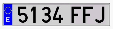
Disregarding the color information, we may see that the objects of this image (numbers and letters) are separated from the background by a stiff gradient:

I0=imread('plate.jpg'); % reading image
I = rgb2gray(I0);       % converting to gray-scale
u=double(I);            % converting to double precission
plot(u(60,:)),title('Intensity function across one horizontal line')

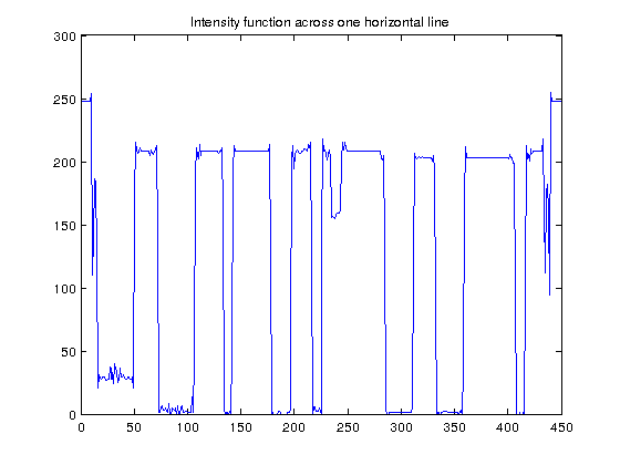
Segmentation algorithms exploit this fact to split the image into regions.

Level sets

Definition of level set. Given a function $F:\Omega\to\mathbb{R}$ the $c-$level set of $F$ is the subset of $\Omega$ given by \( \left\{ x\in\Omega : F(x)=c \right\} \).

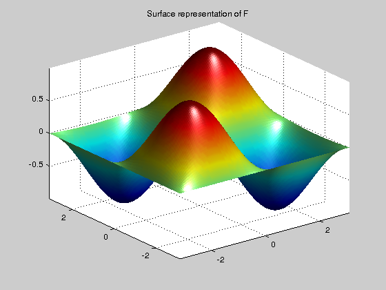
Mathematically, segmented regions are defined by level sets (or contours) of the image

[X,Y]=meshgrid(-pi:0.05:pi,-pi:0.05:pi);
F= sin(X).*sin(Y);
figure,surf(X,Y,F);title('Surface representation of F');
shading interp;camlight;axis tight;                         % for a nicer representation
figure, contour(X,Y,F,10);axis ij                           % draws 10 level sets of $F$
title('Ten level sets of F');

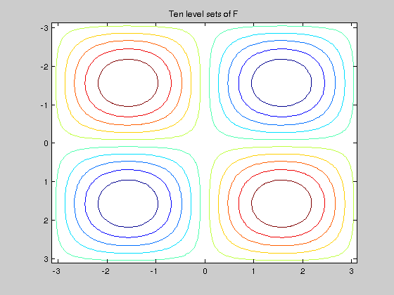
Most segmentation methods uses this fact, being the main idea to start with an initial curve which may (or may not) surround the objects, and make it evolve towards the level sets in which a high gradient separates different regions.

A curve in $\mathbb{R}^2$ is usually defined by a parametrization, i.e. as a function $\gamma: [0,1]\to\mathbb{R}^2$, with $\gamma(t) = (\gamma_1(t),\gamma_2(t))$. But, alternatively, me may define a curve as the level set of a surface, i.e. as \[ \gamma = \left\{x\in\mathbb{R}^2: F(\gamma(x))=c \right\}\qquad\text{for some }F:\mathbb{R}^2\to\mathbb{R}. \] For instance, the following two definitions correspond to the same curve, a circumference: \[ \gamma(t)=(\cos(2\pi t), \sin(2\pi t)), \quad\text{for }t\in [0,1)\qquad\qquad\text{and}\qquad F(x,y)=0, \quad\text{with } F(x,y)=\sqrt{1-x^2+y^2}.\]

Mean curvature motion

The curvature of a surface give us an idea of how far or how close a surface is from being a plane. For instance, the curvature of a plane is zero. And the curvature of a sphere is $1/r$, where $r$ is its radious. Both a plane and a sphere have the same curvature at all their points. But this is a special situation. In general, the curvature of a surface changes from point to point.

Using the curvature to solve physical problems is usual since it is related to how forces apply to objects. Think, for instance, in the design of the nose of an airplane. The curvature of the nose is obviously important. That's why an airplane is not designed as a shoe's box (which would be cheaper).

Let $\gamma$ be the zero level set of some surface described by the function $u_0:\mathbb{R}^2\to\mathbb{R}$. The evolution of $\gamma$ by mean curvature motion corresponds to the minimizing flow of the length of the curve \[ \int_0^1 \|\gamma'(s)\| ds ,\] which is equivalent to solve, for $t>0$ \[\frac{\partial u}{\partial t}(t,x)=-\kappa (u(t,x)) \qquad\text{where}\quad \kappa (u(t,x))=-\|\nabla u(t,x)\| {\rm div} \Big(\frac{\nabla u(t,x)}{\|\nabla u(t,x)\|}\Big)\] with $u(0,x)=u_0(x)$, the initial surface, being $\gamma$ the zero level set of $u_0$.

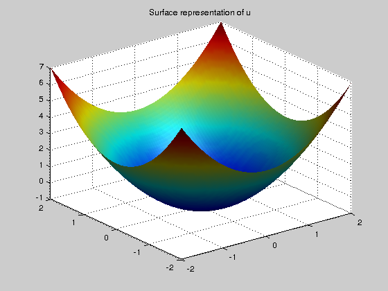
We may solve this problem using the gradient descent algorithm (see Lab 08), \[ u^{(k+1)} = u^{(k)} - \tau \kappa(u^{(k)}).\] Exercise. We make the zero level set of a paraboloid to evolve according to mean curvature. Write the following in a script. We, first, create the surface:

clear all
[X,Y]=meshgrid(-2:0.05:2,-2:0.05:2);
u0 =  (X).^2 + (Y).^2  - 1;                              % The surface is a paraboloid
figure,surf(X,Y,u0);title('Surface representation of u');
shading interp;camlight;axis tight;

Now, we define the time step, the number of iterations and the initial datum:

dt=0.5;
num_iter=200;
u=u0;

Now, we want to implement the loop

%for i=1:num_iter
%	force =kappa(u);
%	u = u+dt*force;
%   plot_level(u0,u,i);
%end;

Here, kappa and plot_level are two matlab function to be created. You can download plot_level.m from the webpage. To write function kappa, i.e. \[ \kappa (u)=-\|\nabla u\| {\rm div} \Big(\frac{\nabla u}{\|\nabla u\|}\Big)\] follow these steps

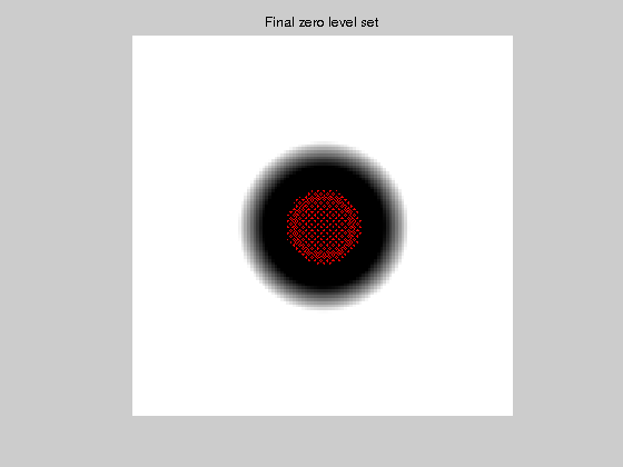
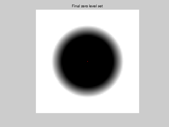
As you can see, the curve follows an inward motion. In the last iterations the curve degrades, due to numerical errors. We shall see how to correct this.

mean_curvature

Redistancing

During PDE resolution, a level set function might become ill-conditionned, so that the zero crossing is not sharp enough. The quality of the level set function is restored by computing the signed distance function to the zero level set. This may be done using the matlab function bwdist. We see here the effect of redistancing

mean_curvature_rd

The Chan-Vese algorithm

Chan-Vese active contours corresponds to a region-based energy that looks for a piecewise constant approximation of the image. The energy to be minimized is \[ \min_{u,c_1,c_2} L(u)+\int_{u(x)>0} | u_0(x)-c_1 |dx +\int_{u(x)<0} | u_0(x)-c_2 | dx\] where $L$ is the length of the zero level set of $u$. The integrals on domains of the type $u(x)>0$ may be expressed through the Heavyside function \[ H(x)=\left\{\begin{array}{ll}1 & \text{if } x>0, \\ 0 & \text{if } x<0, \end{array}\right. \] in the following way: \[ \int_{u(x)>0} F(x)dx = \int_{\Omega} H(x) F(x)dx,\quad \int_{u(x)<0} F(x)dx = \int_{\Omega} (1-H(x)) F(x)dx.\]

The minimizing flow for the Chan-Vese algorithm may be approximated by \[\frac{\partial u}{\partial t}(t,x)=-G (u(t,x)) \qquad\text{where}\quad G(u)=-\nu \kappa (u) - (u_0-c_1)^2 + (u_0-c_2)^2\] Here, we take \[ c_1=\frac{\int_{\Omega} u_0(x) H(u(x))dx}{\int_{\Omega} H(u(x))dx} \quad\text{and}\quad c_2=\frac{\int_{\Omega} u_0(x) (1-H(u(x)))dx}{\int_{\Omega} (1-H(u(x)))dx} .\] and then apply the gradient descent algorithm \[ u^{(k+1)} = u^{(k)} - \tau \kappa(u^{(k)}).\] The program has several technical details which must be solved. You can download a matlab function here, which we shall comment in class. We see some examples

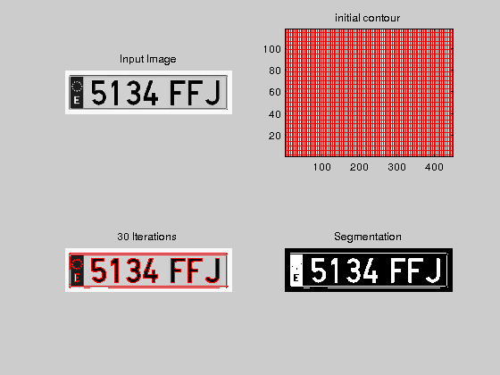
I=imread('plate.jpg');
Fchanvese(I);

Relative error = 9.4162e-05
Convergence achieved

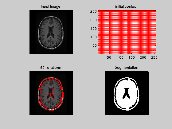
I=imread('IM55.bmp');
Fchanvese(I);

Relative error = 0.00099182
Relative error = 0.0002594
Convergence achieved

Published with MATLAB® 7.6